Creating Accessible Excel Worksheets from Scratch

Saving and Naming the File

Just like with your Word documents and PowerPoint Presentations, you might have your own way of naming your Excel files. However, it’s important to ensure that your Excel files too are named and organized in a way that makes sense to everyone, and keep things crystal clear for all users without the need for lengthy explanations. As discussed in the previous chapters, students are often juggling multiple courses, while working on a single laptop screen. If instructors don’t name their resources clearly and consistently, things can get pretty confusing pretty fast.

How to do it:

• If creating a series of resources for use within a course, consistently use the course name or code as the first item in the name:

“CourseSchedule_Fall2022” becomes “HESA4040_CourseSchedule_Fall2022”

• Follow the course code with the topic, or content, of that specific resource, rather than something like the week of delivery within the course:

“HESA4040_Wk5_Assignment1” becomes “HESA4040_BalanceSheetExercise_Wk5”

• Only abbreviate where there can really be no doubt about the meaning of the abbreviation, particularly when content is for a foundational course early in a program.
• Help students differentiate their notes and files from your resources by including your name or initials early in the name, and encourage them to do the same.
• Avoid including version numbers: it’s not useful information for a student. A date of creation, or date of last edit, is perhaps more useful, but should sit at the end of the file name.
• Direct students to follow the same conventions when submitting their work, and/or creating group project materials, so that we normalise this simple aspect of accessibility across the wider culture.

Finally, when saving a document for the first time, ensure that you do so as a “*.xlsx”

And if saving as a PDF, you will need to take an additional step:

1. In the “Save as type” list, select “PDF (*.pdf)”.
2. Select the “Options” button.
3. Ensure that the “Document structure tags for accessibility” checkbox is selected.
4. Select OK and Save.

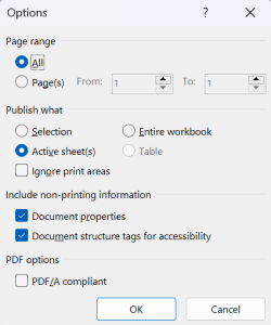
Finally, when saving your document, take a moment to add metadata which includes essential details such as authorship, keywords, and subject headings. More information can be found within this chapter under the following heading: Metadata for Accessibility

Quick-Fire Fact: Need an instant screen reader perspective as you edit your content?

In Microsoft Excel, make use of the Speak feature to swiftly check your content from a screen reader perspective while editing your spreadsheet. By audibly articulating the data, this tool allows you to assess the reading order, ensuring your new spreadsheet is not only visually effective but also accessible to screen reader users.

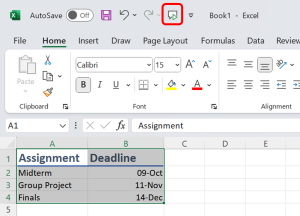
More instructions on activating and using the feature can be found in our chapter: Updating your existing Excel Spreadsheet for Accessibility

Setting up your Worksheet for accessibility

Establishing Logical Reading Order

Logical reading order isn’t just about visual organization; it’s crucial for users who rely on keyboard navigation or screen readers. By establishing a left-to-right, top-to-bottom flow, you enable users to use arrow keys (up, down, right, or left) to navigate your sheet systematically.

How to do it:

1. Always begin your worksheets from cell A1. It’s the equivalent of starting each page at the top-left corner.
2. Refrain from spreading content across multiple rows or columns. This ensures that users can move seamlessly through the sheet without encountering unexpected jumps or disruptions in the reading order.

Setting up Data into Tables

In crafting accessible tables, Excel has an important role as a powerful tool for creating tables, even when the tables are required for your Word or PowerPoint documents. Its data processing and visualization features simplify the table design process, allowing for easy manipulation of data without compromising structure. Once the table is perfected in Excel, it could be imported into Word or PowerPoint, while still preserving the table’s organization and accessibility.

Turning your data into tables is more than just a style choice; it’s a strategic move to enhance the readability, structure, and overall navigability of your spreadsheet.

Creating Header Rows

This setting ensures that a screen reader knows it should treat information in the first row or column differently from the information within the spreadsheet itself: you have to tell the assistive technology that these are titles, rather than data points.

How to do it:

1. Click on the row that contains your header information.
2. In the Excel ribbon, go to the “Table Design”. This tab appears when your cursor is inside a table.
3. Click on the “Header Row” option to designate the selected row as the header row.

Now we’re not going to run through a general ‘how to’ of the Table functions here: a quick online search will bring up instructions of how to use them.  Our focus is on the accessibility functions within Excel tables.  There are a number of things you can do to ensure your Tables are accessible.

1. Make sure the object on the page actually is a Table…this may sound obvious, but if you are copying and pasting a Table from another source, make sure you paste the Table, and not a picture of a table. If unsure on this, you can find instructions online.
2. Keep your table structure straightforward. Avoid complex layouts or merged cells, as they can confuse assistive technologies.
3. Ensure that your table includes clear column headers. These headers serve as the signposts for understanding the content within each column

For more information, and for guidance on how to create more complicated tables, see this guidance from the Web Accessibility Initiative: link to W.A.I guidance (opens in new tab)

The Styles menu

Just as we use “Styles” in Word to structure documents, in Excel, we utilize “Styles” to create a clear and organized structure for our data. This not only benefits users of assistive technologies but also simplifies your work. These styles clarify the purpose of your content, maintain a consistent look and feel across your worksheet, and make it easier for users to navigate.

Utilizing the default styles provided by Excel, such as “Titles and Headings” and should be your initial choice before creating custom styles or directly applying character formatting.

How to do it:

1. Select the first Cell(typically A1)
2. Find the “Styles” command group in the Home tab and select the “Title” style if the worksheet needs to have a title or simply begin with “Heading 1” Style

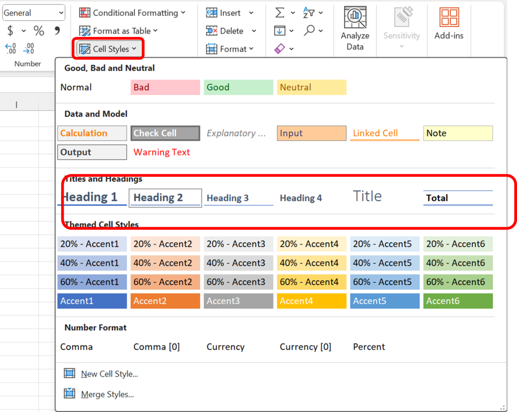
Benefit of utilizing predefined cell styles is that when you make modifications to the formatting linked to a particular style, all the cells that previously used that style will automatically reflect the changes. This eliminates the need for manual adjustments, providing you with an instant preview of how your entire worksheet will appear with the updated format.

Define Names to Range of Cells

In Excel, defining names for specific data ranges within your spreadsheet serves a dual purpose: it streamlines the organization of your data and significantly improves accessibility.

Imagine your Excel spreadsheet as a big city, with each data range representing a distinct landmark. Without named ranges, it’s like exploring this city without street signs – confusing and disorienting. However, by assigning meaningful names to these ranges, you’re effectively installing clear signposts throughout your spreadsheet.

How to do it

1. Begin by highlighting the cells you wish to name, and navigate to the Formulas menu tab, where you’ll find the “Define Name” option in the Defined Names section
2. In the Name text box, give your data range a clear and descriptive name. This name should reflect the content within the range.
3. Then using the Scope drop-down list, specify where this name can be referenced within your spreadsheet.

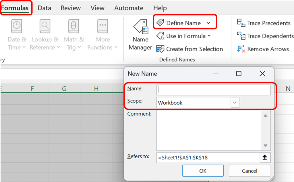
By assigning names to data ranges, you can use the keyboard shortcut Ctrl + G to display a list of all the names defined in your cells. Once you select a specific name from the list and click OK, Excel instantly navigates you to the exact location of that named range within your spreadsheet.

Furthermore, Excel offers a set of advanced functions that, while not essential, can significantly enhance the accessibility of the data. Whether you’re striving for data accuracy with Data Validation, or adding clarity to your spreadsheets with Conditional Formatting, these functions are the bridge between complexity and simplicity, making your spreadsheets an accessible resource for everyone.

Data Validation

Data Validation is your go-to tool for maintaining order in your spreadsheet. It allows you to set the rules for what kind of information can be entered into each cell. Think of it as your spreadsheet’s rulebook, ensuring that your data behaves correctly.

With Data Validation, you can specify the type of data that’s allowed, whether it’s numbers, dates, or specific values. You can also establish limits, such as minimum and maximum values, to prevent any errors. This feature not only makes your data more accurate and consistent but also enhances accessibility, making it easier for everyone to work with your spreadsheet.

For more information, detailed instructions, and steps on how to use Data Validation, you can refer to: Guide on using data validation in excel (external website)

Conditional Formatting

Conditional Formatting is a powerful tool which lets you apply special formatting to cells based on specific conditions, making important data pop out and instantly understandable.

For instance, imagine you have a massive dataset, and you want to highlight certain data points or cells, that’s where Conditional Formatting steps in, making it a easier for everyone to spot trends, patterns, or outliers. You can get creative with font styles, colors, or cell fills based on values, giving your data a makeover. This ensures that all users can effortlessly differentiate and compare different data points.

For more information, detailed instructions, and steps on how to use Conditional Formatting, you can refer to: Guide on using Conditional Formatting in excel (external website)

Enhancing Readability with Colour Contrast

A spreadsheet’s effectiveness should not hinge solely on visual elements, as this can create barriers to accessibility. One crucial aspect to consider is the contrast ratio between the text and the document background – a factor that significantly impacts readability and comprehension. So when you need to use colour formatting beyond black and white for the elements in your presentation, consider the following:

• Envision your spreadsheet without colour—does it still convey the supposed meaning? If not, then you might refer to strategies to incorporate text-based formatting as discussed in the previous sections of this chapter.
• Utilize the Colour Contrast Analyser (external site – opens in new tab) to assess text and other elements in your spreadsheet.
• Based on the contrast result using the analyzer, adjust your font contrast and aim for a minimum contrast ratio of 4.5 : 1 to enhance readability and comprehension.
• Choose contrasting colors wisely, keeping in mind the diverse visual needs of your audience.

Using Images, Charts and Graphs

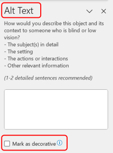
When introducing images, charts or any other graphical objects in the spreadsheet, it becomes important to attach concise alternative text to those objects. If the objects are intricate visuals, such as complex flowcharts, it is advisable to provide a brief text alternative along with a more detailed description.

To add Alt. Text, we can right click on the item and then select the Alt-text option.  If the object is purely decorative, and adds nothing to the meaning of the document, select the Mark as Decorative Object.  In all other cases, use the text box to describe the content of the object.

For detailed guidance on how to capture the meaning in Alt Text, see our dedicated section here: Chapter: Use Alt-Text for Images.

Metadata for Accessibility

To put it simply, metadata, includes details like authorship, keywords, and subject headings, giving the spreadsheet a unique identity and making it easier to locate – the author’s name signifies ownership, while keywords and subject headings act as navigational aids.

How to do it:

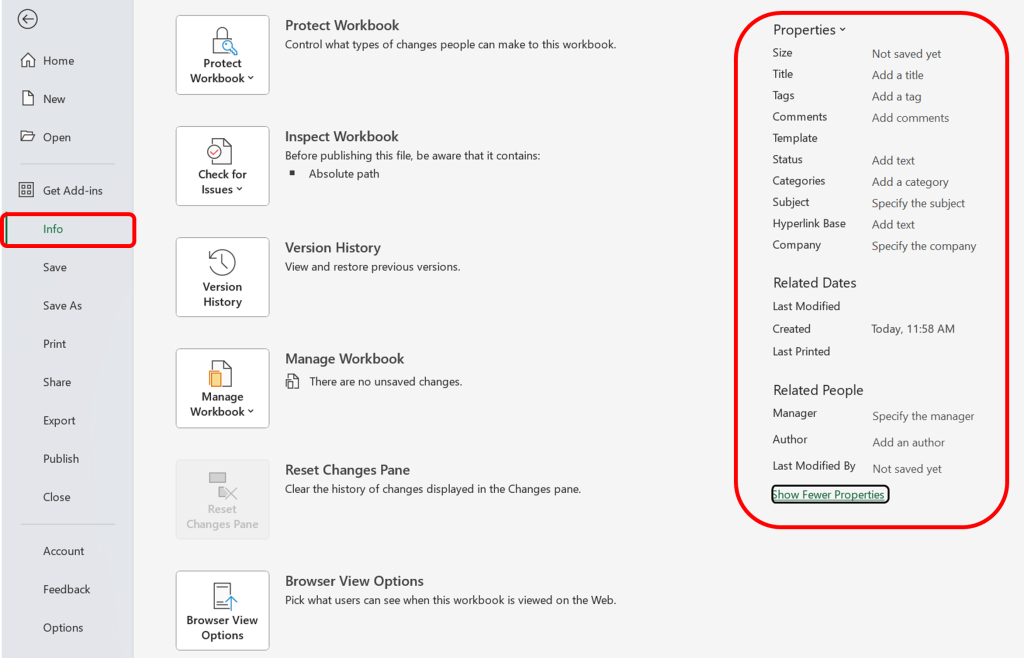
• By clicking on the “File”, navigate to “Info” in the left menu
• Find the “Properties” option at the top right corner.
• Input a descriptive title in the “Title” field. Enter the author’s name in the “Author” field. Input keywords, a brief description, and subject headings in the respective fields, and save the changes.

Using the Accessibility Checker

Word provides a robust tool, the “Accessibility Checker,” to assess the accessibility of your spreadsheet. This feature conducts a thorough review, identifying potential issues that users with disabilities may encounter.

However, it is important to note that the Accessibility Checker cannot always detect all the accessibility issues comprehensively. For instance, while it can identify missing alternative text, it cannot not ascertain if the alternative text is accurate and descriptive. Additionally, it doesn’t test for certain issues, such as color contrast.

How to do it:

• Ensure your file is saved in the “xlsx” format. Older formats may not be compatible with the checker.
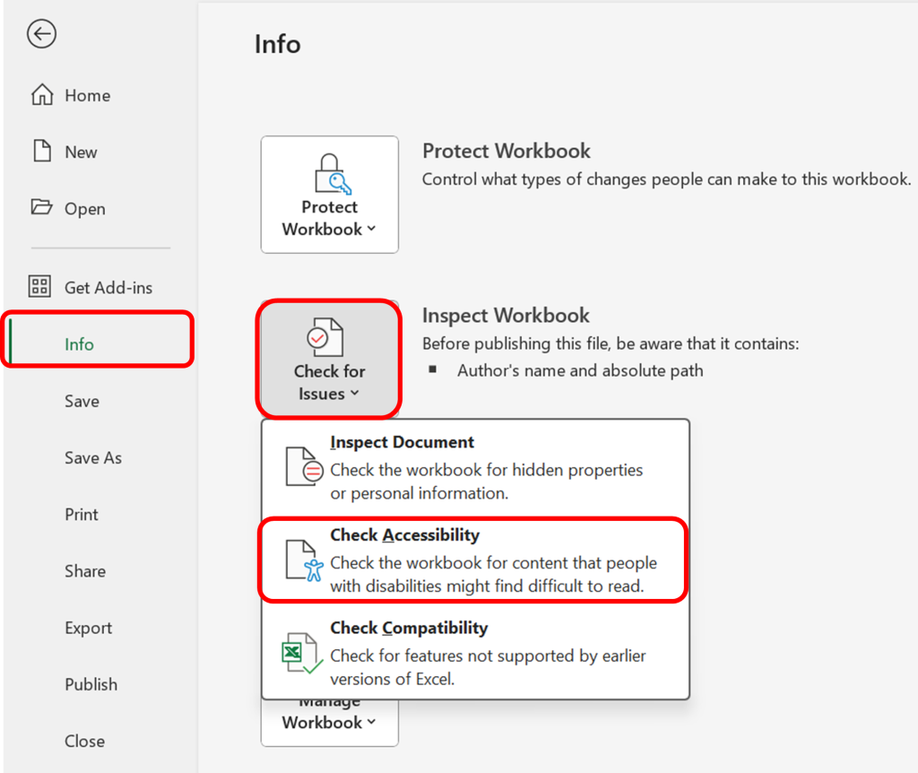
• Navigate to the “File” menu. Under the “Info” section in the left window pane, select “Check for Issues” and then choose “Check Accessibility.”
• A task pane will open, presenting the inspection results.
• Select a specific issue to view additional information and follow the provided steps to rectify or revise the content.

Some of the common accessibility errors and warnings, and information on how to update/adapt your existing Word resources for accessibility can be found here: Chapter: Updating your Existing Excel Spreadsheet for Accessibility

Please don’t hesitate to contact us with suggestions and updates using this: email link for updates(opens in external site/application)

Reference: ED Accessibility Requirements for Electronic Documents | U.S. Department of Education.